Optimal Control Overview
Overview of the optimal control framework and insights into LQR and MPC
Introduction
Control of a system (in our case a robot) is usually done using two paradigms: model-based and model agnostic.
In this post, I will go over the model-based approach, more specifically the optimal control approach.
A diagram showing the main components of this approach is shown in Figure 1. Each component will be analyzed in the sections below.

Follow along example
To get a more intuitive sense, I will explain how to control an autonomous vehicle to follow a reference trajectory $(X, \beta, \psi)$ on a highway.
This task requires controlling both the steering angle and the acceleration of the vehicle.
For simplicity, we will decouple the problem into lateral tracking and longitudnal tracking and focus only on the lateral aspect.
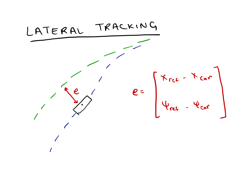
In lateral tracking, the controller aims to minimize lateral offset from a path and keep in the same heading as the reference.
The longitudnal tracking aims to keep the vehicle at a target velocity (mostly constant). As this is ususally done via model-free controllers (PID) and for the sake of simplicity, we will neglect longitudnal control and assume longitudnal velocity for lateral tracking.
A depiction of the lateral tracking (at constant longitudnal velocity) problem is given in Figure 2.

Reference Path
For our reference path, we will be given a set of way points (from an upstream planning module), where each waypoint is $[X_{lateral}, \beta, \dot{\psi}]$. The slip angle ($\beta$) and the heading rate (\dot{\psi}) can be found using the road curvature (which is dependent on the acceleration and velocity of our waypoints)*.
Model of a system
As the name suggests, a model of system to be controlled is needed for this approach to work. This model is formulated using a state space approach.
In this approach, a system of ODE model the evolution of the system in time. Here, the state are the variables which fully describe how the relevant variables we care about change through time.
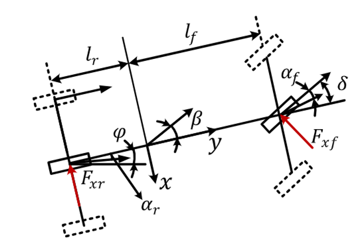
For our example of lateral path tracking, the states are the lateral velocity from the path, and the yaw rate. The model which describes the evolution of these parameters is called the single track, linear dynamic bicycle model (as seen in Figure 3)

In this model, we assume the forces on the lateral (left and right) tires are equally distributed, hence we can collapse the car into a one track bicycle. This assumption is valid for highway driving where aggressive maneuvers are uncommon (slip angle is between 0 to 4 degrees). When aggressive steering and acceleration is needed, a higher fidelity non-linear model is required to account for the uneven force distribution in the tires.
The state-space formulation of this model is as follows:
\[\dot{X} = AX + B\delta\] \[\begin{bmatrix} \dot{x} \\ \dot{\psi} \end{bmatrix} = \begin{bmatrix} -\dfrac{c_{af} + c_{ar}}{um} & \dfrac{-l_f c_{af} + l_r c_{ar}}{u I_{z}} \\ \dfrac{l_f c_{af} - l_r c_{ar}}{um} + u & -\dfrac{l_f^2 c_{af} + l_r^2 c_{ar}}{u I_{z}} \end{bmatrix} \begin{bmatrix} x \\ \psi \end{bmatrix} + \begin{bmatrix} \dfrac{c_{af}}{m} \\ \dfrac{a c_{af}}{I_{z}} \end{bmatrix} \delta\]Change to include the Khajepour paper formulation
As seen, the states evolve in time based on the current state and the steering angle, which is our control input. The objective of our controller is find the steering commands, such that it matches the trajectory. So, we will need a metric which can track this discrepancy, we need a cost function.
Discrete Model Formulation
Continuous formulation of the bicycle model cannot be directly implemented on our digital computer, hence we need to discretize our model. To discretize, we will use Forward Euler numerical integration method. Usually, RK-4 is used but for the sake of simplicity we will use Forward Euler.
The Forward Euler formulation of our model $\dot(x) = f(x,u)$ is as follows for our preview (in our case finite horizon of 5) states $x_k$ and control inputs $u_k$ :
\(v_1 = f(x)\) \(v_2\) \(v_3\) \(v_4\) \(x_{k+1}\)
The predicted outputs are written using these equations for the prediction horizon, based on $x_0$ and the unknown control vector $U$ (to be found after cost optimization).
Cost Function
A cost function (also called an objective or loss function in different literature) is a scalar function which provides a numerical value on the performance of our controller.
Based on how it is formulated, the controller will act differently. Usually, the cost function has the following “quadratic” structure.
\[J = \int_{t = 0}^{T} \left[ \mathbf{\bar{x}}^T(t)\, \mathbf{Q}\, \mathbf{\bar{x}}(t) + \mathbf{u}^T(t)\, \mathbf{R}\, \mathbf{u}(t) \right] dt + \mathbf{x}^T(T)\, \mathbf{Q}_f\, \mathbf{x}(T), \quad \mathbf{Q} = \mathbf{Q}^T \succeq 0, \quad \mathbf{R} = \mathbf{R}^T \succ 0, \quad \mathbf{Q}_f = \mathbf{Q}_f^T \succeq 0.\]In this formulation the $\bar{x}^TQ\bar{x}$ part penalizes the tracking error while the $u^TRu$ part penalizes the control effort (how aggressive you want to steer). The objective of the controller is to minimize this cost function (minimize tracking error and not be too aggressive with steering). Both the $Q$ and $R$ matrices are positive definite, and can be tuned to prioritize tracking over control effort or vice versa. Generally, this is a trial error process.
This cost formulation can be of two types: either finite horizon or infinite horizon. In the finite horizon formulation, the cost accounts for the trajectory in the near future while in the infinite horizon case it considers the entire trajectory. For our purposes we will, stick to the finite horizon case, where $N$ represents the number of timesteps in the future the cost funtion looks forward.
Again, a cost function can be off any form and still be valid, it can include non-linear or higher order terms. But the reason we typically use quadratic costs is because we can gurantee optimal solution using our controller, either numerically or analytically. We have solvers which can solve for control inputs which are the global minimum for our cost function. Hence, the name optimal control.
The first solver which we will look at is Linear Quadratic Regulator (LQR) which finds an analytical for our control input.
Solvers
Linear Quadratic Regulator (LQR)
LQR is one of the solvers/optimizers used to minimize the cost function. It exploits the additive nature of the cost to analytically obtain an equation for the optimal cost.
The optimal control law turns out to be a linear gain applied to the state matrix as shown below.
\[u^* = -Kx\]The gain is derived using the following formulation, where the S(t) matrix is found by solving a Differential Riccati equation.
\[K = R^{-1}B^TS\] \[-\dot{S} = SA + A^TS - SBR^{-1}B^TS + Q\] \[S(T) = Q_f\]Note: I will not go into the derivation of the final result, but interested readers can look into Bellman’s principle of optimality and how it is used to derive LQR control law
This control law is guranteed to be the optimal for this cost formulation for a linear system. For our example, it will work pretty well too, and is a good starting point. But on the road, we want to gurantee safety (prevent aggressive movements) and prevent the vehicle going off the road and hitting someone. The cost function by itself can prevent deviation and minimizes aggressive maneuvers but cannot gurantee it will be within a certain safe limit. Hence, we need to account for constraints.
Constraints
Constraints in the context of optimal control are bounds we set to our state space and control input to keep them within a desirable range. For our example, the constraints might look something like the following.
\(X_{left} \leq X_{pred} \leq X_{right}\) \(\delta_{left} \leq \delta_{pred} \leq_{right}\)
Where the state constraints specify the lane boundaries we want to be within, and control constrainsts specify the steering angle limits of our vehicle we cannot exceed.
We do not want our control values from our controller and the resulting states of our system to be outside this range under any circumstance, we need a gurantee on these bounds.
It turns constraint makes our lives much messier and there does not exist an analytical way to optimize our cost function. We must rely on numerical optimization and that is where we turn to Model Predictive Control (MPC) for assistance.
Model Predictive Control (MPC)
MPC is a more general optimal control framework which accounts for constraints. It does so by leveraging numerical optimization techniques like Quadratic Programming (QP) and Convex Programming (CP).
Both QP and CP are out of the scope of this article, but suffice to say they will find the global minimum solution if the cost is quadratic (for QP) or convex (for CP).
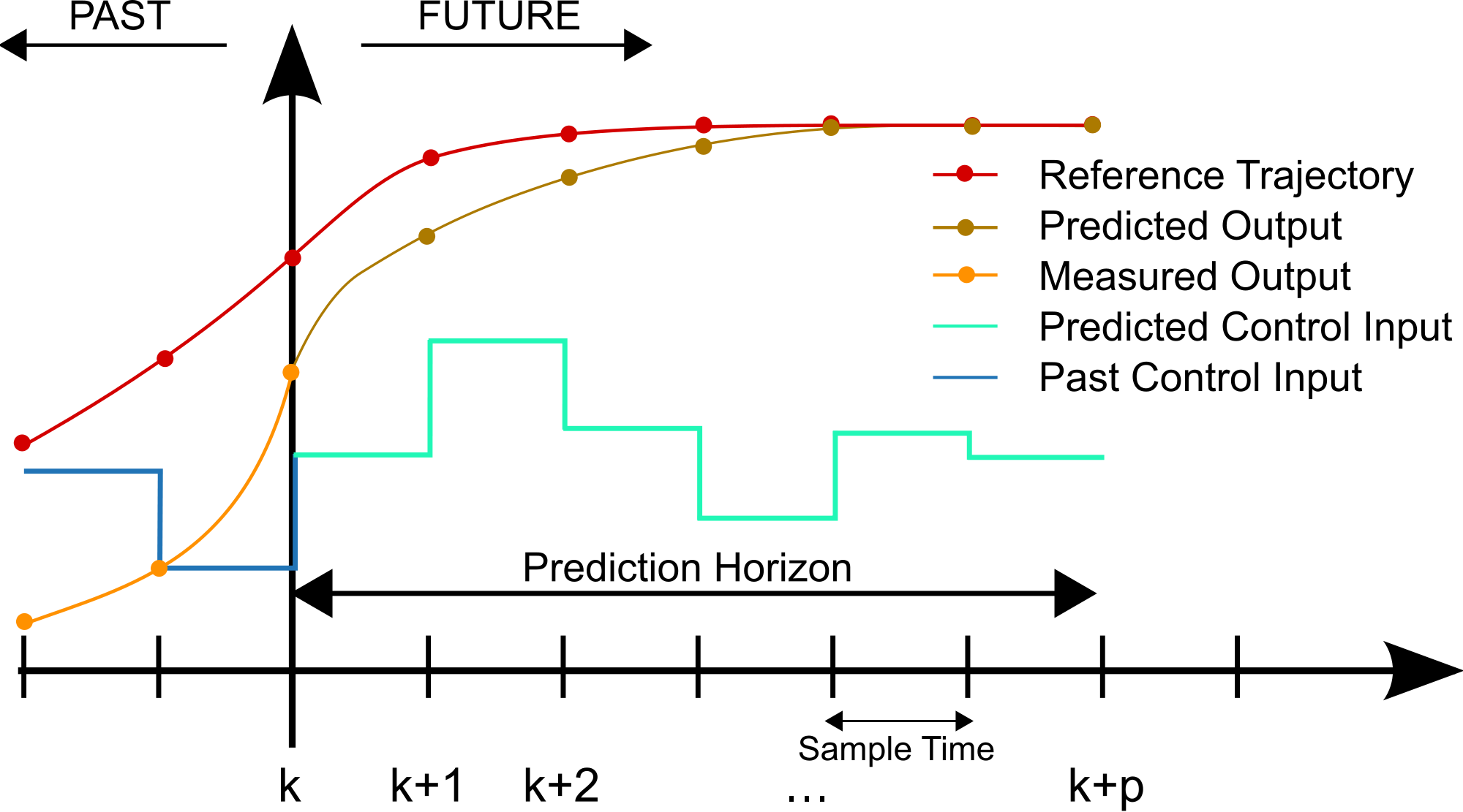
Using these solvers, MPC the optimal predicted trajectory and it’s associated control inputs and selects the first one to be sent to the actual vehicle (a depiction is shown in Figure 4). This process is then repeated in the next timstep.

Given numerical optmization is required in MPC, it takes more compute then LQR but with the advances in hardware, real-time operation is possible.
Miscellaneous
This section is dedicated to things to keep in mind when implementing optimal control on a real system:
- Need to have a discrete-time formulation of the model.
- When discretizing never use Forward-Euler (use RK4)
- Make sure the parameters of the model match the parameter of the car.
- Make sure the model assumptions hold valid for the car.