Lyapunov Functions, foundation of nonlinear system analyis.

History of Lyapunov Functions and applications to control theory and robotics.

Introduction

Non-linear systems are notoriously hard to analyze and finding a solution trajectory for such systems is usually analytically intractable and numerically expensive. Even the numerical solutions have artificats in them, and do not give the global picture (ex: global stability) of the system. Therefore, a formal way of analyzing the gloabl behavior of such systems was needed and that was fulfilled through the concept of Lyapunov functions.

What are Lyapunov Functions?

Lyapunov functions referered to as $V(x)$ are positive definite for all states ($x$) of the system, execpt when $x = 0$, and the time (or the lie derivative) of $V$ ($\dot{V}(x)$) is less than or equal to $0$. To write the conditions more formally:

\[V(x) \succ 0, \forall x \ne 0 \tag{1}\] \[-\dot{V}(x) \succeq 0, \forall x \tag{2}\]

If you can find such a function for a system, you can conclusively make claims about the stability of the origin. For example, if $\dot{V}(x)$ is strictly negative and the domain of the lyapunov is the domain of the system, then the system is globally asymptotically stable (all trajectories eventually converge to the origin). If $\dot{V}(x)$ is semidefinite in the domain, then the origin is stable (or Lyapunov stable), meaning if a point starts of “near” the origin, it will stay “near” the origin as the system evolves with time. Again, if the domain is the entirety of the system domain, then the origin is globally stable.

If the domain is a subset of the system’s domain, the we can only say that the origin is locally stable/asymtotically stable for $V(x) \leq \rho$.

As a side, if a function does not satisfy $(1)$ and $(2)$, then it does not mean the system is unstable. We can draw no conclusions from such a function.

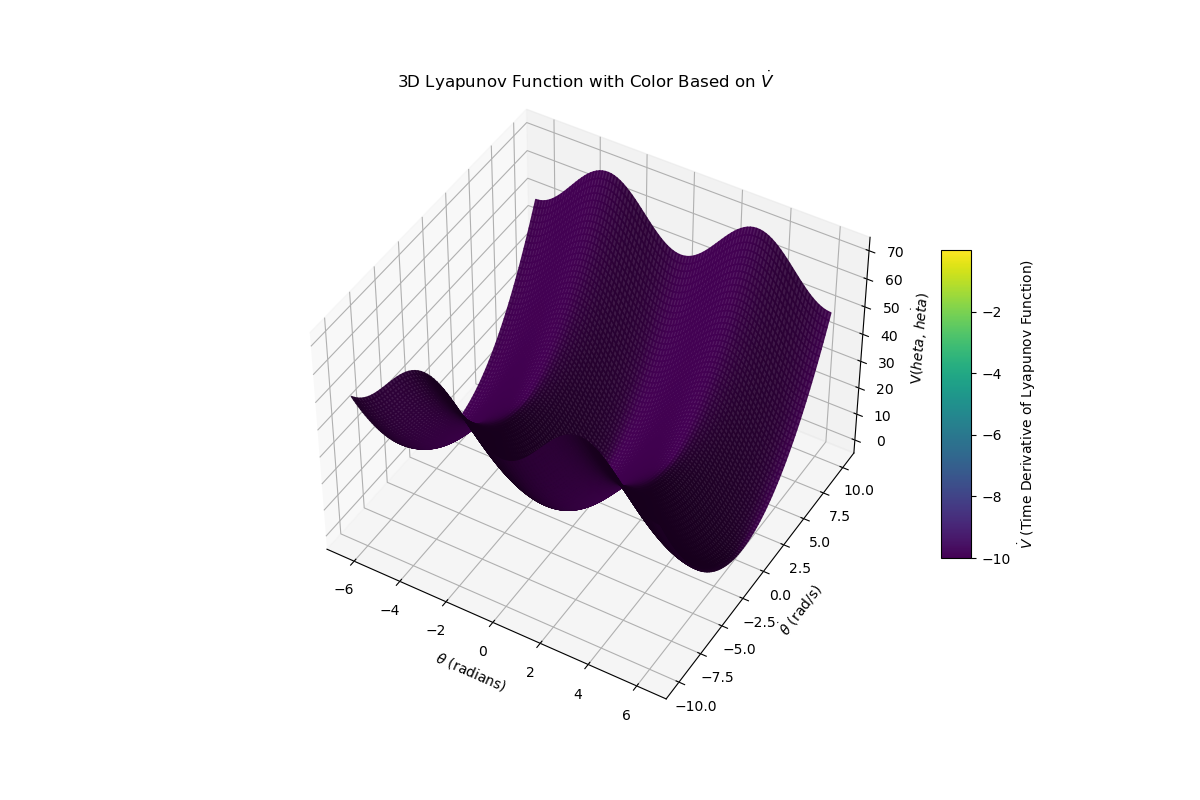
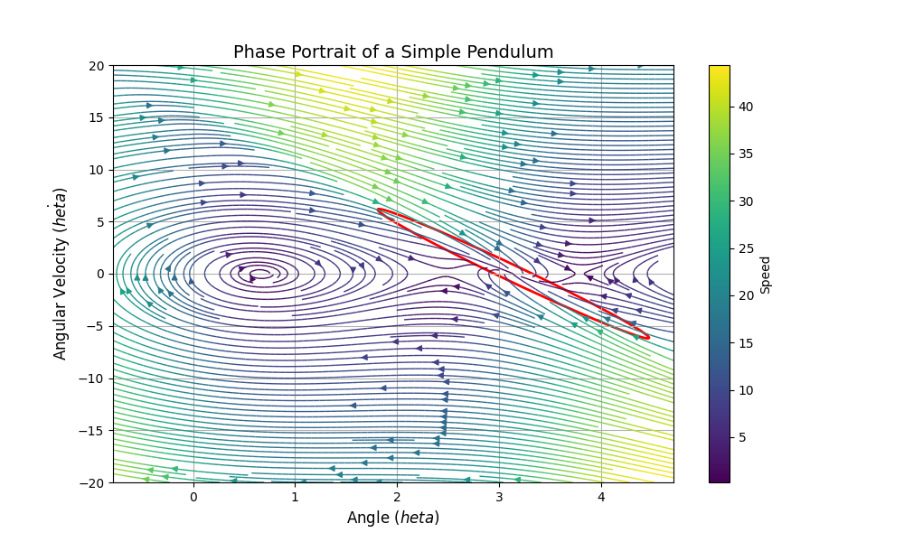
One way to think about Lyapunov functions is to compare it to the concept of Energy. Actually, one suitable Lyapunov candidate functions for mechanical system is energy as seen through the example in Figure 1.

Figure 1: Total Energy Lyapunov function for inverted pendulum system where the color represents the time derivative of Lyapunov. As energy meets requirements (1) and (2), the origin is globally asymptotically stable.

Computing Lyapunov Functions

Typically, for most systems (even those physical in nature) it is hard to find a lyapunov function which can give conclusive evidence regarding the stability of the system. Other candidates usually used are quadratic functions of the form: $V(x) = x^TPx$ where $P \succ 0$. This form usually requires trial and error to find the correct coeffecients of $P$ for non-linear systems, while for linear systems you can use Semi-Definite Programming (SDP) to find $P$ from Lyapunov’s Equation. This methodology can be extended to non-linear system thorough linearization, but provides extremely conservative estimates for the region of attraction (local regions where the trajectory of a system converges to a point $x_o$).

If the non-linear system is polynomial (or can be closedly approximated as a polynomial), sums-of-squares programming can be used to find $V(x)$ of usually quadratic or quartic power. This method was applied to the control of the inverted pendulum in the LQR-Trees paper . In this paper, the cost-to-go $J(x)$ of a linear quadratic regualtor (LQR) was used as the Lyapaunov candidate function for a closed loop system at a goal point and SOS-programming was used to find the largest sub-level set ($V(x) \leq \rho$ where $\dot{V}(x) < 0$) as an estimate of the region of attraction. Figure 2 shows the Region of Attraction estimate of the inverted pendulum problem at $(0, \pi)$ using SOS programming.

Figure 2: Region of Attraction estimation using Lyapunov Functions for the inverted pendulum with satuator constraints.

In reality, polynomial approximation of systems can be quite restrictive and numerical issues can arise during the optimization process where Lyapunov conditions can be violated. Furthermore, SDP and SOS programming scale poorly with number of states in the system, limiting them to low-dimensional systems. Even some provem globally aspymoptotically stable systems, have no polynomial Lyapunov function associated with them. Hence, more generalized representations of Lyapunov functions are needed which are scalable i.e. time to use Neural Networks!

Neural Networks as Lyapunovs

As nerual networks are universal funcion approximators, it is only natural to use them to learn Lyapunov Candidates for a system. With neural networks you are not restricted to simple quadratic/quintic representation of Lyapunov function, the possibilities of functions to consider are virtually endless. Many in academia have used neural networks to learn lyapunov functions of the system as well as the control policy simultaneously. More detailed information of the parameterization of the networks can be found in the survey paper by Dawson .

Most of these formulation have the same structure, a neural network to learn a Lyapunov function and a controller (with a cost function to optimize towards the Lyapunov conditions) and a verifyer to check whether the learned function meets the Lyapunov requirements. Typically, the check is done offline after training using SDP, Mixed Integer Programming (MIP) or Satisfiability Modulo Theories (SMT) solvers. These solvers are expensive to use for verification, hence this process is not done online.

For example, in , the lyapunov is initialized randomly and the controller network is initialized witht the LQR solution. Without loss of generality, the loss function can be losely defined as follows:

\[L(\theta, u) = V_{\theta}(0)^2 + max(0, -V_{\theta}(x)) + max(0,\nabla_{f_u}V_{\theta}(x))\]

In this loss formulation, if all the lyapunov conditions are satisfied then the loss will be zero, else it will be positive. The training process utilizes training by counter-examples and it is as follows:

A random state is sampled uniformly in the state space
The $V(x)$ and $u(x)$ are calculated
Loss is calculated for $V(x)$
If loss is greater than 0 (Lyapunov conditions are violated)
The parameters of $V(x)$ are updated via gradient descent
Process continues until convergence (certain amount of steps for which loss is 0 consecutively)

In this training process, you can get a probabilistic certainty that the $V(x)$ does not violate the lyapunov conditions, but since then, other paper have been published which utilize formal solvers to check network and generate counter-examples for further training of the network until convergence. If no more counter-examples can be produced by the formal solver, then the network is lyapunov and the corresponding controller guarantees stability .

But what about the region of attraction? How do you get an estimate of that using the trained Lyapunov function. This is still and open area of research, one method starts of with a small bounded region, trains the lyapunov function until convergence, and iteratively keeps expanding the box until convergence seems infeasible. In the largest box on which convergence was possible, the largest sublevel set of the trained $V(x)$ is taken as the estimate .

This general methodology of finding Lyapunov functions has made it easier to find larger ROA (2 to 5x the size) on non-linear control problem benchmarks like the inverted pendulum, vehicle path following and quadrotor hovering. Still, this method has its drawbacks. Even though it scales better than SOS methods and has been applied to systems with dimension 8, going beyond that still is an open problem. Furthermore, the solver are expensive to compute online and have to be done offline, so if the enviornment (dynamics) changes, the training and verification would have to be done again offline *.

Applications

Even with the limitations of finding and computing Lyapunov functions for nonlinear systems, they have been applied successfully to a wide variety of problems. Some of these applications are briefly described here.

LQR-Trees

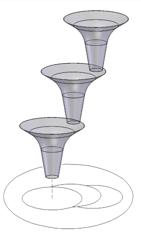
LQR-Trees is a feedback motion-planning algorithm for state bounded non-linear systems. This algorithm produces a policy for each state in the system. This algorithm utilizes the idea of funnels (as seen in Figure 3) to gurantee stability/tracking when travelling between two states. As long as the state starts inside the funnel, it will end at the goal state which is the output of the funnel. These funnels can be sequentially composed to cover the entire state-space and reach the goal point from any state as long as the state space is bounded.

Figure 3: Sequential Funnels for motion planning .

The “funnel” to a goal point from a set of initial point requires the use of Lyapunov functions in it’s creation. In the paper, between two points, a trajectory generation algorithm (like direct collocation) is used to get a trajectory of states and control inputs. For each of the state-input pair, the discrete algebraic ricatti equation is solved backwards (for the LQR problem) to get a cost-to-go and optimal control action. The cost-to-go is selected as the Lyapunov function for the close-loop dynamics and a SOS problem is solved for the trajectory of cost-to-go’s to create a funnel which gurantees that any point starting in the funnel stays in it and eventually converges to the goal point (outlet of the funnel).

Using these “funnels” and RRT, LQR-Trees probabilistically covers the state-space offline for a given state space and at run-time it takes in the intial state and outputs control actions until the system reaches the goal state. Detailed treatment of this algorithm can be found in the paper .

Funnel libraries

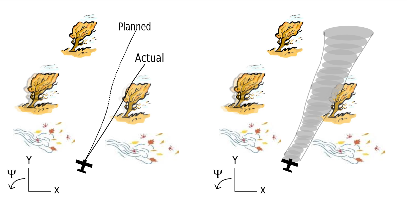
Unlike in LQR-Trees, Lyapunov functions are used as a safety gurantee in this work . In this work, a library of motion primitives of the desired system is created and a funnel for each of these primititves is computed offline. Unlike LQR-Trees, the aim is to create these funnels as “tight” or “small” as possible to minimize the worst-case reachable set of the system.

During runtime, the optimal funnels are chosen from the libraries and are sequentially composed to operate the system in a safe manner in unseen enviornments. A depiction of how the algorithm operates on a plane is depicted in Figure 4.

Figure 4: (a) Plane Deviation from nominal trajectory (b) "Funnel" of possible trajectories .

Control Barrier Functions

Control Barrier functions (CBFs) can be thought of as the transpose of Control Lyapunov functions (CLFs). While CLFs focus on the stability of dynamical systems, CBFs focus on the safety aspect. Unlike CLFs, CBFs do not require the restrictive Lyapunov conditions, they only need invariance condition $\dot{h}(x) \geq 0$ (where $h(x) \geq 0$ defines the safe set $C$) on the boundary of a subset as shown in Figure *. Hence, CBFs can be though of as a superclass of CLFs, where all CLFs are CBFs but not all CBFs are CLFs.

Therefore, CBFs are defined a bit differently as follows :

\[sup_{u \in U}(L_fh(x)+L_gh(x)u) \geq -\alpha(h(x))\]

Where $h(x)$ replaces $V(x)$ and is not necassarily positive definite, just $h(x) \geq 0$ for the safe set. In this formulation, $h(x) = 0$ at the boundary and $\alpha$ is a strictly increasing function with $\alpha(0) = 0$ that prevents $\dot{h}(x)$ from going negative too quickly (prevents infinite slope). Quadratic Programming (QP) is generally used find the controller $u(x)$ for CBF given an initial controller, the QP is formulated as follows :

$u(x) = argmin_{u \in R^m} \frac{1}{2} ||u-k(x)||^2$ $s.t. L_fh(x) + L_gh(x)u \geq -\alpha(h(x))$

If there are no input constraint, then a closed form solution can be obtained (min-norm controller), else a numerical solution is obtained. This can be combined with CLF constraint to get a multi-objective optimization problem (known as QP-CBF-CLF), where both stability and safety are solved for simultaneously, although a relaxation term is needed on stability to gurantee safety. Usually, the control inputs are of a higher relative degree, hence exponential CBFs are introduced to find solutions for such control inputs.

QP-CBF-CLF for safe trajectory optimization has many applications such as automatic cruise control and lane keeping, dynamic walking, etc .

###