Variational Inference

Introduction to how Generative models work

The blog post is based primarily on the excellent overview paper by Calvin Luo, for detailed treatment of proofs and implementation check out his paper .

Intro, Surprise, and Cross-Entropy

• Probability is the degree of belief ( a measure of confidence rather then frequency)
• Probability Distribution is a function that maps the state to its probability
• Sampling: generating samples from the underlying distribution. How to do this for complex distributions?
• Surprise: measure (function of probability) which is high for rare events (high surprise) and low for common events. When probabilities multiply, the surprise should add. The function that behaves this way is the logarithm of \(\frac{1}{p_s}\).
• Can charecterize entire distribution by it’s average surprise. This average (expected) surprise is known as the entropy of the distrubution and has the following formula: \(H = \sum_s p_s log(\frac{1}{p_s})\)
  • Interpretation: measure of inherent uncertainty of a distribution when predicting.
  • In real world, we do not have access to the true distrubtion, we use an internal approximate model (our belief about the distribution).

Cross Entropy

• What if the deviation between the internal model and the actual model is significant?
  • Cross Entropy: function of two probability distribution, which quantifies the average surprise you will get by observing a RV from dist. P, while believing in its model Q.
  • The formula is as follows: \(H(P,Q) = \sum_{s}^{states} p_s log(\frac{1}{q_s})\)
  • High Surprise can come from two sources: believing the wrong model or the inherent uncertainty of the process. Believing in the wrong model, can only increase surprise not decrease it.
  • \(H(P,Q) != H(Q,P)\) <- Assymertical ->

KL Divergence

• KL Divergence: $H(P,Q) - H(P) = \sum_s p_s log(\frac{p_s}{q_s})$
  • It measures the surprise casused by the model and true distribution being different (extra surprise), beyond the uncertainty of the true distribution itself.
  • Why measure this?
    • Good for learning distributions of images (in ML)
    • For autoencoders
      • Loss function: KL-Divergence make as low as possible to make the output distribution as close to the input.
      • Usually, framed as minimizng cross-entropy (means the same thing as H(P) is constant). Therefore, KL-Divergence can never go to zero.

Variational Inference

• How to build and utilize world models from partial information?
  • Use variational inference
• Describing complex underlying distrubution effectively with limited sampling.
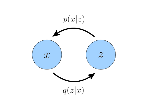
  • Observation (x) will be determined by a hidden latent variable (z) with its own distribution P(z).
  • Latent variables can be though using Plato’s Allegory of the cave. Some underlying variable which influences the observations.
  • No need to find it, let the model learn it.
  • For a given z, find the $P(x\mid z)$.
  • Joint probability is: $P(x, z) = P(z) * P(x\mid z)$.
• How to represent distribution?
  • Use points? Too cumbersome
  • Use parameteric approach: represent dist. with few key parameters. Ex: Gaussian Distribution (only 2 parameters)
  • For multi-dimensional data use the higher dimension joint gaussian version (Covariance matrix and mean vector)
  • NN can output these 12 numbers but will cause problem in higher dimensions.
  • Common assumption: covariance matrix is fixed, isotropic gaussian, only mean needed to be outputted by the NN.
  • NN is outputting the parameters of the prob.distribution. Hence, for a sample $z$, we out a probability $P(x\mid z)$.
• Objective is to minimize the error (some distance) between distribution $P(x), P_\theta (x)$
  • Minimize KL Divergence -> maximize $\sum_x^{states} P(x) log P_\theta (x)$
  • But true data distribution is unknown, but we have access to finite sample (our dataset)!
  • Allows us to approximate the expectation over the true underlying distribution using a simple average.
  • Now, estimate $P_\theta (x)$ -> we can get $P_\theta (x\mid z)$ using latent to outputting distribution parameters.
  • Many different z values could have generated a specific x value, so need to consider all possible latent values: $P_\theta (x) = \sum_z P_\theta (x\mid z)P_\theta(z)$ (called likelihood)
  • Hence, model allows needs to learn the parameters of the prior (distribution of z)

Training loop in a nutshell to learn model distribution from samples (given we know P(z))

1. Take a data point (x) from training dataset
2. Randomly sample many candidate $z_k$ from the distribution $P(z)$ (prior already known, what if we don’t know?)
3. Map each $z_k$ through the NN and get parameters for the $P_\theta(x\mid z_k)$ for each $z_k$.
4. For each $z_k$ compute the $P_\theta(x\mid z_k)$
5. Compute average log-likelihood $log[\sum_z^{z_k} P_\theta (x\mid z)P_\theta(z)]$
6. Iteratively update (using gradient descent) $\theta$ to maximize the log-likelihood across the dataset.

Higher-Dimenstional latent space and Evidence lower bound

• Curse of dimensionality: sampling grows exponentially with number of dimensions for adequate coverage.
• But most latents don’t explain the data
• Use importance sampling!
• Better to oversample rare and important cases, and mathamatically correct for the bias, rather then risk missing them entirely!
  • How to find these “important” regions in the latent space
  • Instead of blindly sampling from the entire latent space, we train a seperate neural network to do this!
  • This network learns to predict which region in the latent space have likely generated each data point.
    • NN leans a variational distribution: $Q_\theta (z\mid x)$
  • Can try optimize the parameters of $Q_\theta$ and $P_\theta$ directly by maximizing: $log P_\theta (x) = log E_{z~Q_\theta (z\mid x)} [P_\theta (x\mid z) \frac{P_\theta(x\mid z)}{Q_\theta(z\mid x)}]$ but is probelematic.
  • Fundamental issue is the log of the expectation (average) is hard to optimize (noisy and unstable).
• Jensen’s Inequality:
  • \[log E[X] \geq E[log X]\]
  • Hence, by swapping the possition of expectation and log from our objective above, we can get a lower bound on our objective (Evidence lower bound -> ELBO). If we maximize this lower bound, we automatically maximize our objective.
  • Computationally, much easier to maximize ELBO.
  • Has intuitive meaning for the terms:
    • Accuracy term : $E[logP_\theta(x\mid z)]$
    • Complexity term: $D_{KL}[Q_\theta(z\mid x)\mid \mid P_\theta(z)]$

Implementation Notes about the prior $P_\theta (z)$

• In theory, can learn the distribution of the prior distribution.
• But typically, prior is fixed to be an isotropic gaussian, with zero mean and identity covariance.
• Only learn the weight of the recognition model $Q_\theta(z\mid x)$ and the generative model $P_\theta (x \mid z)$

Updated Training loop

1. Take a data point (x) from training dataset
2. Pass through NN of recognition model to get the parameters of the importance sampling model $Q_\theta(z\mid x)$.
3. Use the $Q_\theta$ distributon to effectively sample ($z_k$)from the $P_\theta(z)$ prior distribution.
4. Map each $z_k$ through the NN and get parameters for the $P_\theta(x\mid z_k)$ for each $z_k$.
5. For each $z_k$ compute the $P_\theta(x \mid z_k)$
6. Compute the ELBO objective (which is to be maximized): \(E[logP_\theta(x\mid z)] - D_{KL}[Q_\theta(z\mid x)\mid \mid P_\theta(z)]\)
7. Iteratively update (using gradient descent) $\theta$ to maximize the ELBO objective across the dataset.

Note: both recognition and generative model do not output the distribution directly, just the parameters. So have to put these into the formula for the gaussian directly to get samples.

The accuracy formula in ELBO is proportiaonal to the following: $log P_\theta (x \mid z) ~ - \mid \mid x-\mu \mid \mid ^2$ with the isotropic gaussian assumption!

Also the KL-divergence term (using this gaussian assumption) in ELBO can also be calculated using only the model parameters, hence ELBO is an ideal objective for training, as literal sampling each step is not required.

Variational Autoencoders (VAE)

• In the default VAE formulation, ELBO is directly maximized.
• Typical autoencoder: encoder and decoder
  • Latent space $Q_\psi$ is smaller then the observation space
  • Observation (input) data is trained to predict itself after undergoing an intermediate bottlenecking representation step (latent).
  • Each input $x$ results in a distribution over possible latents $Q_\psi(z\mid x)$
  • This distribution of latents is converted into an output observation using a learnt deterministic decoder $P_\theta (x \mid z)$.
• ELBO is optimized jointly over $\psi$ and $\theta$. THe encoder $Q_\psi(z \mid x)$ is usually a multivariate Gaussian with diagonal covariance and the prior $P(z)$ (our assumption of the true distribution of the latent) is often standar multivariate Gaussian. $Q_\psi (z \mid x) = \mathcal{N} (z; \mu_\psi (x), \sigma_\psi^2 (x) I)$ $P(z) = \mathcal{N}(z; 0 , I)$
• The reconstruction term in ELBO is maximized using Monte Carlo estimates while the divergence term is calculated analytically.
  • Stochastic sampling is non-differentiablem, hece reparameterization trick needed to be able to differentiate the parameters. $z = \mu_\psi (x) + \sigma_\psi (x) \epsilon$ $\epsilon ~ \mathcal{N}(\epsilon; 0, I)$
• After training, generating new data is performed by sampling directly from the latent space $P(z)$ and then running it through the decoder.

Hierarchical Variational Encoders (HVAE)

• Generalization of a VAE that extent to multiple hierarchies (layers) over latent variables.
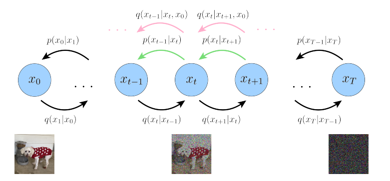
• Markovian HVAE: each transition in the hierarchy is Markovian. Decoding each latent $z_t$ only conditions on the previous latent $z_{t+1}$.
  • Basically stacking VAEs on top of each other. (recursive VAE)

Figure 1: VAE depicted by the arrows: the forward arrow is the encoder ($q(z \mid x)$) which defines a distribution over the latent $z$ for observation $x$; and the backward arrow is the decoder ($p(x \mid z)$) which defines a distribution over the observation $x$ for some sampled latents.

Variational Diffusion Models (VDM)

• VDM is mVAE with 3 restrictions:
  1. Latent dimension is exactly equal to the data dimension
  2. Structure of the latent encoder at each time step is not learned, it is predefined as a linear Gaussian model. (Gaussian dist. centered around the output of the previous timestep)
  3. The Gaussian parameters of the latent encoders vary over time in such a way that the distribution of the latent at timestep T is a standard Gaussian.
• In VDM, we are only intreseted in learning the decoder conditionals $p_\theta(x_{t-1} \mid x_{t})$ so that we can simulate new data. The encoder distribution $q(x_t \mid x_{t-1})$ are no longer parameterized by $\psi$, instead are completely modelled as Gaussians with defined mean an variance parameters at each timestep.
  • The encoder transitions are defined as: \(q(x \mid x_{t-1}) = \mathcal{N} (x_t; \sqrt{\alpha_t}x_{t-1}, (1-\alpha_t)I)\)

Figure 2: VDM as a hierarchy of forward and reverse diffusion processes. The aim of the diffusion model is to minimize the difference between the distribution between the pink (Gaussian noise corruption step) and the green (denoising step) arrows.

• After optimizng, the sampling procedure is sampling Gaussian noise from $p(x_T)$ and iteratively running the denoising transitions $p_\theta(x_{t-1} \mid x_{t})$ for T steps to generate a novel $x_0$.

• Using reparameterization trick recursively, along with markov and gaussian assumptions, the optimization objective simplifies to the following:

\[\arg\min_{\theta} \; \mathbb{E}_{t \sim \mathcal{U}(2, T)} \left[ \mathbb{E}_{q(x_t | x_0)} \left[ D_{\mathrm{KL}} \big( q(x_{t-1} | x_t, x_0) \; \|\; p_\theta(x_{t-1} | x_t) \big) \right] \right]\]

• The above stochastic optimization objective can be interpreted as finding the parameters (of a neural network) that minimizes the expected KL-Divergence between the true reverse diffusion process and our learned reverse process.

• The outer expectation during training can be replaced by randomly sampling different data points from the (training) dataset.

• The inner expectation can be replaced by uniformly sampling different noise levels (timesteps t).

  Three interpretations of the $D_{KL}$ term:

Reconstructing the ground truth image

• One way to break down the $D_{KL}$ term is as follows:

• Here, optimizing the VDM boils down to learning a neural network to predict the original ground truth image from an arbitrarily noisified version of it.

\[D_{\mathrm{KL}} \big( q(x_{t-1} | x_t, x_0) \; \|\; p_\theta(x_{t-1} | x_t) \big) = \frac{1}{2 \sigma_q^2(t)} \frac{\bar{\alpha}_{t-1} (1-\alpha_t)^2}{(1-\bar{\alpha}_t)^2} \left\| \hat{\mathbf{x}}_\theta(\mathbf{x}_t, t) - \mathbf{x}_0 \right\|_2^2\]

Predicting source noise

• Here, we learn $\epsilon_\theta^hat (x_t, t)$ which is a neural network that is trying to predict the source noise $\epsilon_0 ~ \mathcal{N} (\epsilon; 0, I)$ that determines $x_t$ from $x_0$.

• The objective $D_{KL}$ is now framed as:

\[D_{\mathrm{KL}} \big( q(x_{t-1} | x_t, x_0) \; \|\; p_\theta(x_{t-1} | x_t) \big) = \frac{1}{2 \sigma_q^2(t)} \, \frac{(1 - \alpha_t)^2}{(1 - \bar{\alpha}_t) \alpha_t} \left\| \epsilon_0 - \hat{\epsilon}_\theta(x_t, t) \right\|_2^2\]

Score-based optimization

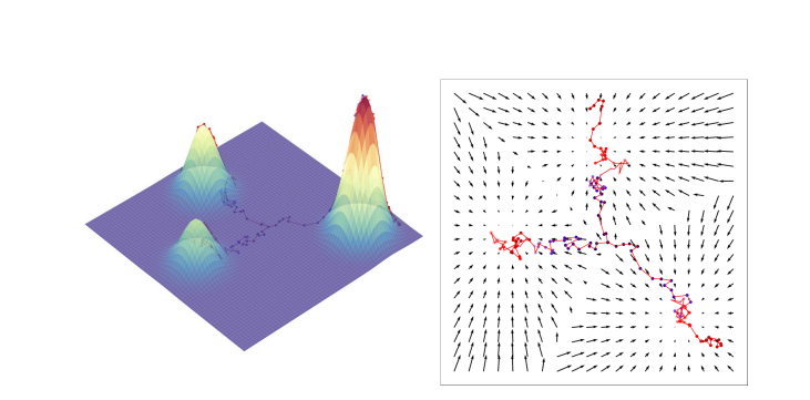
• The third way is to estimate $s_\theta (x_t, t)$ which is a neural network that learns to predict the score function $\nabla_{x_t} log p(x_t)$, which is the gradient of x_t in data space, for any arbitrary noise level t.

• The objective $D_{KL}$ is now framed as:

\[D_{\mathrm{KL}} \big( q(x_{t-1} | x_t, x_0) \; \|\; p_\theta(x_{t-1} | x_t) \big) = \frac{1}{2 \sigma_q^2(t)} \, \frac{(1 - \alpha_t)^2}{(1 - \bar{\alpha}_t) \alpha_t} \left\| s_\theta(x_t,t) - \nabla log p(x_t) \right\|_2^2\]

NOTE: Here, \(p(x) = q(x_t \mid x_0) = \mathcal{N}(x_t; \sqrt(\bar{\alpha}_t)x_0, (1- \sqrt(\bar{\alpha}_t)I))\) is called Denoising Score Matching (DSM)

• To generalize score-based generative diffusion models to infiite timesteps, represent the evolution of the perturbation of the image as a stochastic differential equation (SDE).
  • Sampling is then performed by reversing the SDE

Figure 3: Score based interpretation of the diffusion optimization objective. Optimizing for the score is like moving to one of the modes in the distribution at each time step. The log gradient step defines a vector field along which a randomly sampled data with evolve in time until it converges to one of the modes.

Conditional Guidance for Diffusion Models

• To explicitly control the data we generate through some information $y$ (ex: text, or low res image), we also need to learn the conditional distribution. This forms the backbone of image-text models and super-resolution models.

• Natural way to add conditioning is simply alongside the timestep:

\[p(x_{0:T}) = p(x_T) \prod_{t=1}^{T} p_\theta(x_{t-1} \mid x_t, y)\]

• “Guidance” is needed to more explicitly control the amount of importance the model gives to the conditioning information at the cost of sample diversity.

Classifier Guidance

• The conditional ground truth score can be expanded (using Bayes Rule) to:

\[\nabla log p (x_t \mid y) = \nabla log p(x_t) + \nabla log p(y \mid x_t)\]

• The adversarial gradient term $\nabla log p(y \mid x_t)$ is represented as a classifier that takes in arbitrary noisy $x_t$ and attempts to predict conditional information $y$. The classifier is seperately learnt.
• The score of the unconditional diffusion model $\nabla log p(x_t)$ is learned as previously described.
• During sampling procedure, the overall score function is computed as the sum of both.
• For finer control (either to encorage or discourage the influence of the conditional), a hyperparameter term is introduced:

\[\nabla log p (x_t \mid y) = \nabla log p(x_t) + \gamma \nabla log p(y \mid x_t)\]

Classifier Free Guidance (much more robust in sample diversity, and flexible)

• No need to train a seperate classifer.
• Learn both conditional and unconditional diffusion models together as a singular conditional model.
• The conditional ground truth score then simplifies to: \(\nabla log p (x_t \mid y) = \gamma \nabla log p(x_t \mid y) + (1- \gamma) \nabla log p(x_t)\)
• During training, model is trained on conditional data and unconditional (the conditional information query is replaced with empty string).
  • This is usually done by randomly dropping the condition during training (conditioning dropout).
  • The model learns to denoise both with and without conditioning.
• During the sampling (generation) phase:
  • Run model with no conditioning and with desired conditioning
  • Combine the two predictions using the above weighted average.